Improving HBase's Stochastic Load Balancer

On June 11, 2017, I had the honor of delivering a talk at HBaseCon 2017 alongside my colleague James Moore, from HubSpot. In my portion of the talk, I described my open-source contributions to HBase’s stochastic load balancer. This post will re-cap those contributions for anyone who enjoys learning about complex systems, without requiring any knowledge of HBase. For that reason, this post will start with the basics.

What is HBase at a high level?

HBase is a distributed non-relational key-value database based off of Google’s Big Table. When I say HBase is based off Big Table, I really mean that HBase is essentially an open-source implementation of Big Table. Though, somewhat confusingly, the name HBase comes from the fact that it was originally called the Hadoop Database because it was written on top of the Hadoop Distributed File System (HDFS). For both the keys and the values, HBase only stores uninterpreted byte arrays, as opposed to your traditional types like Integer, String, Boolean, etc. This means that if you looked at the keys in a random HBase table, you’d just find bytes like [0x466a1b1b, 0xa761c388, …] instead of a string value like “cat”. While this may at first seem confusing, it gives HBase the flexibility to store anything that can be represented as bytes (aka everything that can be stored on a computer).

Although HBase is a key-value store, it imposes some structure on how you store the data, unlike a blob store that may let you, say, associate keys with arbitrary blobs of data. In HBase, each table is made up of an arbitrary number (though often small) of column families. Each column family is made up of an arbitrary number (which may be quite large) of column qualifiers. A column qualifier stores several cells. A cell stores a single piece of data, very similar to the usual definition of the word column in a SQL database, along with a version (aka timestamp). The number of versions you store for each column qualifier is configurable. You can choose to store up to n versions of a particular column qualifier, or define an arbitrary TTL (time to live) of the data (i.e. one week, two months, etc.). The table is broken into rows, each of which has a row key which is mapped to a particular set of column families, column qualifiers, and cells.

To picture this, it can be helpful to imagine this structure as nested JSON. It should be noted that this is NOT how the data is actually stored on disk, but this view is helpful for understanding what tables, row keys, column families, column qualifiers, and cells are.

In this example, the Employees table has employee_id as a row key. personal_information and professional_information are column families. And the various fields like home_address, home_phone_number, work_phone_number, etc. are all column qualifiers. We can see that each column qualifier stores multiple versions of each piece of data. This allows you to query HBase for the last three phone numbers of a particular employee, for instance.

Employees table:

employee_id: {
  personal_information: {
    home_address: {
      version: 1, value: ...,
      version: 2, value: ...
    },
    home_phone_number: {
      version: 1, value: ...,
    },
    social_security_number: {
      version: 1, value: ...,
      version: 2, value: ...,
      version: 3, value: ...,
    },
    ...
  },
  professional_information: {
    work_phone_number: {
      version: 1, value: ...
    },
    title: {
      version: 1, value: ...
    },
    salary: {
      version: 1, value: ...
    },
    ...
  },
  ...
}

HBase partitions the data by row key into regions. Regions are then each assigned to a region server. Region servers can host multiple regions, and usually we want all the region servers in the cluster to host an equal number of regions. In the employee example, maybe we’d have one region for all employees whose employee_id starts with 0, one region for all ids that start with 1, etc. One issue with this setup, however, would be the classic thundering herd problem. That is that reading all employee data in sorted order would cause individual region servers to be overwhelmed with requests while the rest of the cluster is idle. For this reason, row keys are usually some sort of hashed value so that sequential reads of all employees whose employee_id starts with 0 won’t all hit the region server who hosts that region.

To make sure that regions are well-distributed among region servers, HBase leverages a component called the Stochastic Load Balancer (which I’m just going to call the balancer from now on). The balancer’s primary function is to, well, balance the cluster. Because my contributions to HBase are all about the balancer, I’ll now describe a bit about how the balancer works.

How does the stochastic load balancer work?

The stochastic load balancer assigns regions to region servers. It does so in a way to bring the cluster to balance.

How is balance defined? Well it’s actually defined in terms of several cost functions. These cost functions each take in the current state of the cluster and output a value between 0 and 1 to assess the state of the cluster. Each cost function assesses a different aspect of the cluster state. There is one cost function, for instance, that makes sure each region server has an even number of regions. There is another cost function that tries to make sure that individual region servers don’t host too many hot regions (i.e. regions that receive a lot of requests).

To find better region assignments, the balancer also defines several generator functions. These generator functions take in the cluster state and propose actions for the cluster to take. An action could be to move a region from one region server to another, swap two regions from two region servers, or do nothing at all. Different generator functions are defined to optimize different goals. As would make sense, many of the cost functions have an associated generator function which tries to optimize the same goal.

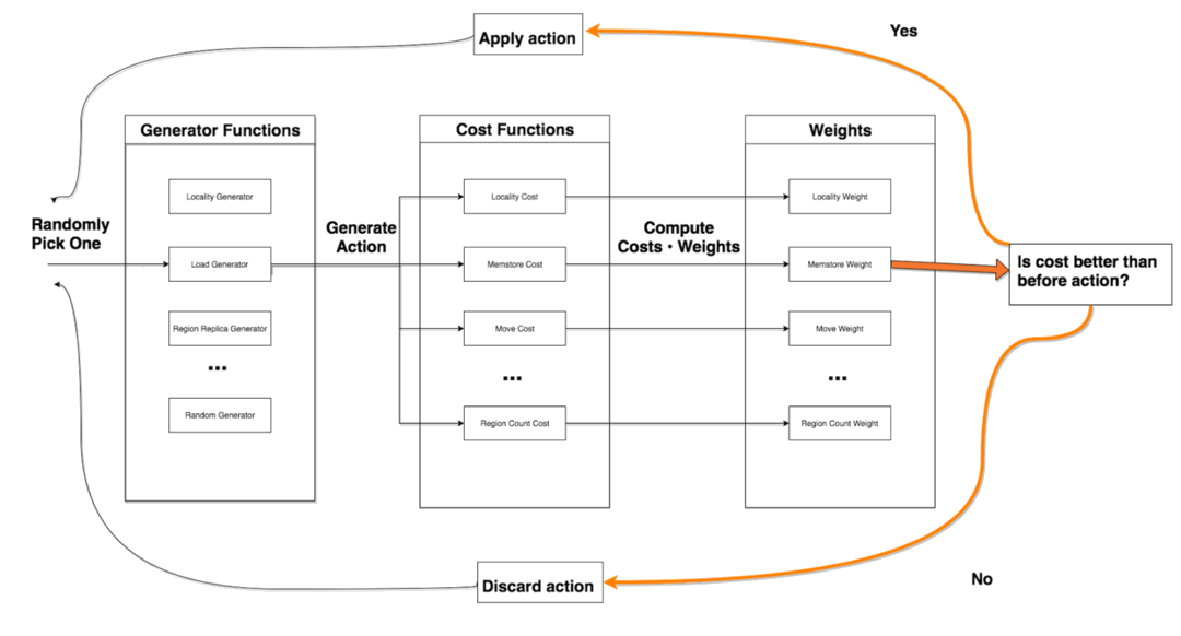
Every n minutes (configurable, but defaults to 5), the balancer runs for m seconds (configurable, but defaults to 30). During these m seconds, it iterates through the following balancing algorithm.

1. Randomly select a generator function
2. Use the generator function to generate an action based on the current cluster state
3. Feed the generated action into all of the cost functions to assess it
4. Accept the action if it brings down the cost of the cluster, or reject it if it increases the cost
5. Repeat 1-4 until m seconds are exhausted.
6. Apply all accepted actions to the cluster

This algorithm can be visualized with the following diagram:

What did I improve?

Issues with Table Skew

We noticed that our HBase clusters suffered from bad table skew. Table skew is when the regions for tables are not well-distributed across the cluster. As an example, consider the following situation:

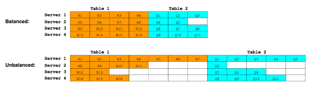
In this image, each row represents the regions stored on each particular region server. We can see that in our unbalanced scenario, Server 1 stores regions R1-R7 for Table 1 and regions Q1-Q5 for Table 2. Not only does Server 1 store more regions than other servers, but it stores proportionally more regions for each table. If we assume each region of Table 1 is accessed equally as frequently, then a disproportionate of requests for Table 1 will be processed by Server 1. This will cause Server 1 to become overwhelmed under heavy workloads for Table 1.

The balancer is supposed to balance table skew. In other words, we would have liked for each server to store 3-4 regions for each table, but instead we see some servers store far more and some store far less. This will lead to general hot-spotting and not allow us to best use the resources in the cluster.

Improving table skew computation

To start, I re-wrote the TableSkewCostFunction, because the old one contained some critically flawed logic. There also was no TableSkewCandidateGenerator, so I wrote a new one. The new TableSkewCostFunction works by computing the minimal distance of the current cluster state from the ideal cluster state, with respect to table skew. With regards to table skew, the ideal cluster state is one in which the regions from each table had been evenly distributed (essentially round-robin-ed) across each server in the cluster. The farther the current state is from the ideal state, the higher the cost value that the cost function outputs. The TableSkewCandidateGenerator simply generates actions that reduce the distance to the ideal cluster state.

Between the two of these, we were able to better analyze and, perhaps more importantly, eradicate table skew from our clusters. The effects were palpable. Here is a graph of the 75th percentile queue times for our region servers. This is a useful metric of how long requests to HBase take. Because this graph is of the 75th percentile, 75 percent of all requests times were better (meaning lower) than the values in the graph while 25 percent were worse (meaning higher).

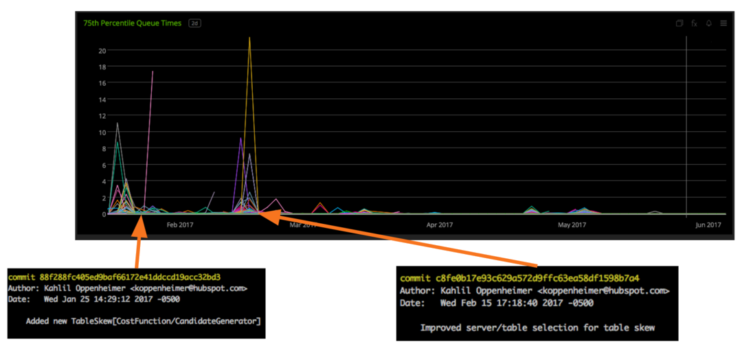
As you can see, after we deployed our new table skew logic (first commit) and a crucial bug we soon after (second commit), our 75th percentile queue times dramatically dropped down, and have stayed down since. For perspective, this graph spans five months.

These changes have dramatically increased the stability of our HBase clusters.

Balancer does not scale with cluster size

We noticed the balancer considers 20x less actions in our big clusters (~100 of tables, ~150 of region servers, ~15k regions, ~300 TBs of uncompressed data) than our small clusters. Because of this, our big clusters often have trouble reaching balance quickly. Because we lose ~3.5% of all of our region servers each month due to hardware failures, and often scale up our clusters by adding new region servers, balance is very important for us to maintain. Without balance, we suffer more usage-related region server crashes and other behavior we’d like to avoid.

We benchmarked all cost functions and candidate generators to get a sense of what was taking so long. We visualized what percentage of the balancer’s computation time was being spent in each cost function (depicted on the left) and in each generator function (depicted on the right). Here’s what we found.

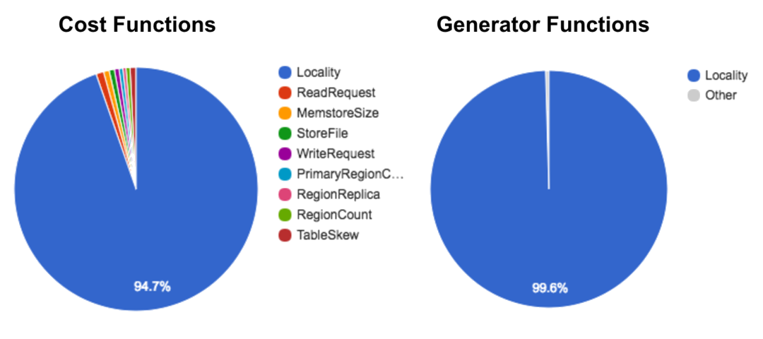
It turned out that the locality computation (both the cost function and the candidate generator) was taking up about 99% of the computation time. Locality is a measure of how close the data is to the computation. For HBase, this translates to how much of a region’s data is present on the disk of the region server on which it’s hosted. Notably, the data for a region is incrementally written to disk as its region server processes requests, rather than when the region is intially assigned to the region server. This makes re-assigning regions have a relatively cheap initial cost, albeit at the cost of lots of incremental work down the line.

Improving locality computation

The old locality computation was very inefficient. At every iteration of the balancer, the old locality computation recomputed the locality of every region on every server. This meant reading the HDFS blocks of every region of the cluster, which is extremely expensive.

Instead, the new locality computation only incrementally updates its cost estimate based off of the most recent region actions. This way, at each iteration of the balancer, it need only look up the locality of at most two regions, rather than every region in the cluster.

Furthermore, the new locality cost function also outputs a slightly different number than the old cost function. The new cost function outputs a value that represents how good locality currently is compared to how good it could be, given the current cluster state. That is to say that if a region is assigned to the region server for which that region’s data is the most local, the cost associated with that region will be 0, even if the region is only a small percentage local on that region server. I believe this more accurately represents an actionable goal for the balancer in regards to locality. The balancer will try to find ways to assign regions where they are most (or at least more) local, rather than just assign high costs when regions are not very local in the cluster.

The results of the new locality logic yielded a 20x performance improvement for our big clusters and a 3-5x performance improvement for our small clusters in the number of actions considered by the balancer. Because the new locality computation takes so much less time, the balancer has more time to think, and can thus more quickly bring the cluster to balance.

Lastly, I added a new type of locality computation: rack-aware locality. For us, this is important because a rack is an Amazon Web Services (AWS) Availability Zone (AZ). There is actually a higher cost associated with inter-AZ data transfer than intra-AZ data transfer. This new cost function allows us to associate a balancer cost with the very real financial cost of transferring data between AZs.

Conclusion

In summary, it has been an absolutely wonderful experience to be able to work directly in the HBase code base. I am honored to be able to contribute back to such a cool and powerful project.